Engr Help

Potential Function (Velocity Potential)

Key Concepts: For the special case of steady, inviscid, incompressible, irrotational fluid flow

a function, φ, called the velocity potential exists. It can be used to simulate fluid flows of

interest by superimposing the potential functions for special cases such as uniform flow, sources,

sinks, doublets, and free vortices.

In a Nut Shell: For steady, inviscid, incompressible, irrotational fluid flow the vorticity vector, ζ ,

is zero. Then there exists a velocity potential, φ, that automatically provides zero vorticity where

u = ∂φ/∂x, v = ∂φ/∂y, w = ∂φ/∂z . Recall

ζ = curl V = (∂w/∂y - ∂v/∂z) i + (∂u/∂z - ∂w/∂x) j + (∂v/∂x - ∂u/∂y) k

Substitution of the velocity components into the above expression for vorticity confirms that

it sums to zero. Substitution of u = ∂φ/∂x, v = ∂φ/∂y, w = ∂φ/∂z into the continuity equation

∂u/∂x + ∂φ/∂y + ∂w/∂z = 0 (continuity equation)

yields ∂²φ/∂x² + ∂²φ/∂y² + ∂²φ/∂z² = 0 ( Laplace equation )

In elementary fluid mechanics emphasis is on two-dimensional fluid flow in the x-y plane.

∂²φ/∂x² + ∂²φ/∂y² = 0

Note that this equation is linear. So that if both φ₁(x,y) and φ₂(x,y) satisfy this equation so

does φ₁(x,y) + φ₂(x,y) which gives a convenient way to superimpose potential functions

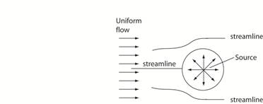
to simulate different kinds of fluid flows. An example might be simulating fluid flow around

a circular cylinder where you superimpose the potential function for uniform flow plus the potential

function for a fluid source as depicted in the figure below.