Finite Volume Analysis: Application
of Conservation of Linear Momentum
|
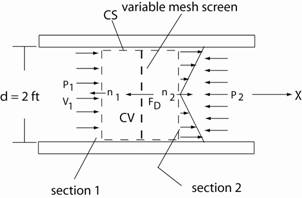
Example 1 (continued) The figure (Step 1 in strategy) below
shows the control volume, control surface, uniform pressures at sections 1
and 2, uniform velocity profile at section 1, linearly distributed, axisymmetric velocity profile at section 2, drag force, FD, exerted by the
screen on the air, the outward unit normals, n1 and n2, the diameter, d, of the circular duct, and
the positive X-axis.
d/dt ∫ ρ dV +
∫ ρ V ● n
dS
= 0 cv cs Since
the flow is steady (established flow)
d/dt ∫ ρ dV = 0.
cv The
flow crosses the control surface at sections 1 and 2. So the second term becomes ∫ ρ V1 ● n1 dS1 +
∫ ρ V2 ● n2 dS2 = 0 cs1 cs2 Now
the uniform velocity profile at section 1 is V1 i and the unit outward normal n1
= - i So V1
● n1 = -
V1 Also assume that ρ = constant So
∫ ρ V1 ● n1 dS1 = -
ρ V1 (π d2/4) cs1 Click
here to continue with this example. |
Copyright © 2019 Richard C. Coddington
All rights reserved.